SITL vs physical servo output differences

I’m trying to create a process to validate that the system dynamics of the attitude controller is the same in SITL and physical hardware.

For the SITL side I am using the MATLAB/JSON interface to simulate the body rotating. I noticed some unwanted randomness on the angle reported in the GCS so I dropped the RND parameters for attitude sensors to zero. That model is available here. I’m still working on it, but this version helps illustrates the issue I am having so far.

For the physical side I have a Cube Black on its own (nothing except USB plugged in) that was calibrated against a flat table. I made a rocking block to make setting the angles easier and snappier to emulate what the SITL model does. I can hold the block flat on the table and then pivot it to the angle that want without having to read anything on the fly.

All parameters relating to the attitude controller (or as far as I can read from the code) and the scaling there of were kept the same (ARSPD_USE=0). Arming checks passed and flight modes were kept to FBWA. The curious thing is that the servo outputs are different. Tridge made a comment about the controller be rate based so to double check myself I cut the rate that the SITL model was using to reach the desired attitude by 4 and got the same result at steady state.

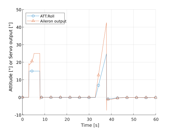
Here is SITL rolling to 15 deg at 200 deg/sec max rate.
plot-validation-SITL-roll

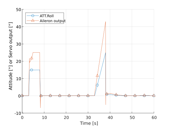
Here is SITL rolling to 15 deg at 50 deg/sec max rate.
plot-validation-SITL-roll-002

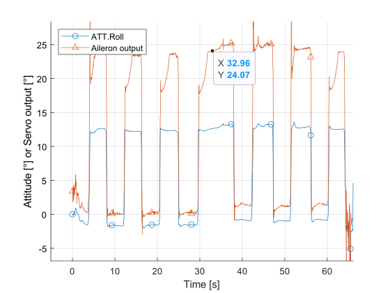
Then here are the physical tests. I did the same thing twice to check my sanity.

First physical test.
plot-validation-physical-roll

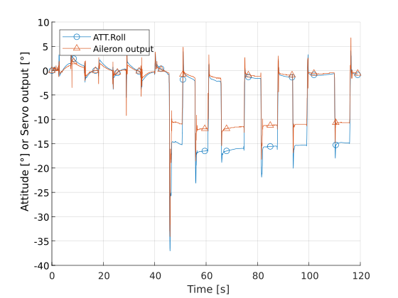
And the second physical test.
plot-validation-physical-roll-002

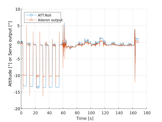
The angle that the physical test gets to isn’t the most consistent or a very clean input signal, but I am working on that. The bigger issue that I am seeing is that the STIL servo output is more than double that of the physical for nearly the same input signal.

Logs that each of these plots were created from are here.

Going to do a quick update now and then I’ll make another more complete update with a cleaner method to do this by parameter changes. After talking with @peterbarker and @tridge they pointed out that the physical test without the gps lock was going to cause a problem since that goes down a different code path for the speed scaler. (Sidenote: PR for logging speed scaler by Peter B) Using the fakegps module in MAVProxy fixed that right up.

The output is now exactly the same! Well pretty close. Tridge suggested fixing up not having the perfect attitude angle can by changing the AHRS_TRIM_* parameters. Which honestly would have been way easier than making the MATLAB model.

plot-validation-physical-roll-003

1 Like

This took a few tries to get the scaling speed to match. That seems to be the trickiest part to match with the gps lock and airspeed estimate.

AHRS_TRIM_X and AHRS_TRIM_Y changes were pretty easy to do. So here is a quick and dirty procedure. I’ll have some more details in my thesis, but if someone else would like to do this and is having difficulty following what I am doing just ask.

Physical side:

  1. Calibrate accel. Reboot to apply values.
  2. Connect to MAVProxy. Load and use the fakegps module.
  3. Pass all arm checks (wait for the EKF to get the fake GPS worked into the math) and arm.
  4. Param show the current AHRS_TRIM* values.
  5. Param set the shown value with the desired rotation in radians.

SITL side: (I think this should work with any SITL backend, but I’m not 100% sure on that.)

  1. Pass all arm checks and arm.
  2. Param show the current AHRS_TRIM* values.
  3. Param set the shown value with the desired rotation in radians.

After that I pull up both logs and double check that the AETR.SS values are the same. Then you just have to compare the RCOU.Cx values. You could also check PIDx.x and AETR.x for efficacy.