Greetings devs. In this post I attempt to make a tutorial/guide for how to use the system identification toolkit for transfer function and state space model estimation.
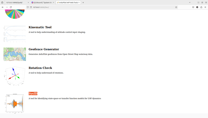
Since the toolkit is part of ardupilot webtools, it can be locally run on the system. The sysID toolkit is in the dev section of the webtool
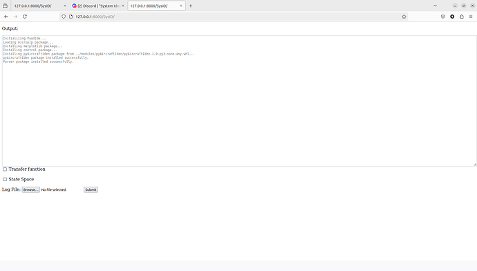
Upon loading, the output screen looks as follows:
The model type that needs to be estimated can be selected from here and then after inputting the identification parameters, log file can be submitted.
State Space Identification
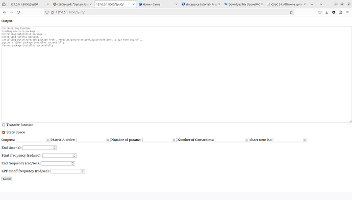
Upon clicking the statespace model a window as shown below appears:
The functions of parameters visible above are as follows:
- Outputs: Number of output data fields that need to be taken from the log
- Matrix A order: Order of matrix A. Order of state space matrix should be equal to number of states in your state space, with shape of A matrix being n X n. The matrix B will always have a shape n X 1, where n is the order of A.
- Number of params: Number of unknown parameters in the state space matrices that need to be identified.
- Number of constraints: Number of equality constraints required by the user. These constraints enforce the condition of two unknown params either always being equal to each other or negative of each other.
- Start and End time: These are for specifying the start and end time of sysID experiment in the log. Only data between these times will be considered while estimation of the model.
- Start and End frequency: Since current webtool relies on frequency response to estimate the system, the start and end frequency specify the region of frequency spectrum from which data will be considered. This should be chosen carefully to capture both short term and long term dynamics of the system.
- LPF cutoff frequency: Before identification, the input and output data is passed through a low-pass-filter to remove noise. The desired cutoff frequency is inputted here.
Once these parameters are submitted, further parameters can be set:
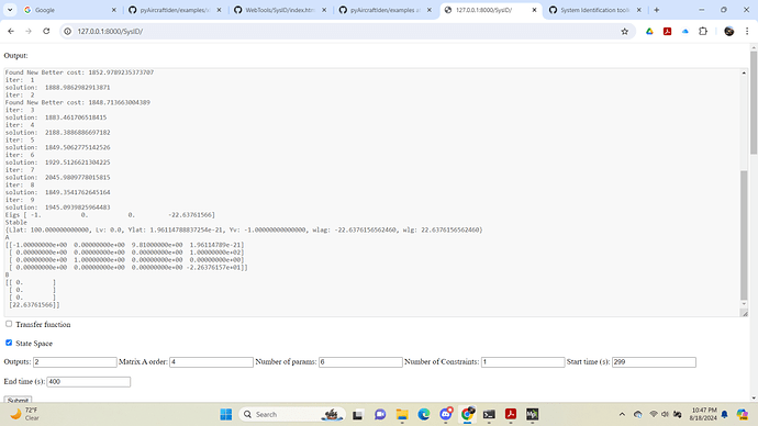
This image shows an example value of parameters filled for identifying the roll state-space model of an x8 configuration UAV.
Upon submission, following parameters pop out:
The functions of parameters visible above are as follows:
- Input: Msg name and field of input data
- Output(n): Msg name and field for nth output
- Multiplier: This is an optional field which can be used to multiply the data with a constant. This can be used for unit changes (for eg: SI to imperial)
- Gravity Compensation: This is a special field for IMU acceleration data along roll and pitch axis. Since IMUs do not measure gravity, the effect of gravity component g*cos(angle) does not get reflected in imu data. To counter this, gravity compensation adds a gravity dependent term (g x theta x multiplier for roll axis or -g x theta x multiplier for pitch axis) to the acceleration data.
- Param(n): Symbolic name to be assigned to nth unknown param
- Bounds(n): The min and max value that the nth unknown parameter can take
- Matrix A: System matrix with shape n X n, with n being the number of states. The known elements of matrices are given there respective values and unknown elements are given there respective symbolic names as inputs.
- Matrix B: Control matrix with shape n X 1. Same principal as A for inputs
- H0 and H1 matrices: These denote the relationship between frequency response variables and the states of the system. In above example, the statespace has four states [velocity_y (Uy), roll rate(p), roll angle(phi), motor lag(w)]. The H0 matrix denotes the states for which data is available. H1 matrix denotes the states whose first derivative data is available
After these parameters are set, the log can be uploaded and submitted.
Since we are currently using a python code running on browser using pyodide, a lot of capabilities of pyAircraftIden are limited, leading to very long solution times for large systems. This is something that I hope to change in future.
Once the processing is complete, the plots become available for comparing the original data and identified system:
The plot shows phase and amplitude fit for both the output values. The final model and numerical fit are displayed on the output screen.
Transfer function estimation
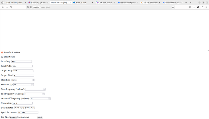
Transfer function estimation has a relatively simple setup and a less computationally expensive process. The output screen for tfestimation looks like this:
The function of each input block is as follows:
- Input Msg and field: Msg type and field for input data
- Output Msg and field: Msg type and field for output data
- Start and End time: Denote the start and end time of the sysID experiment
- Start and End frequency: Denote the region of frequency spectrum in which response is calculated
- LPF cutoff frequency: Cutoff frequency of low pass filter
- Numerator and Denominator polynomial: Since polynomial structure can be dynamic, users need to input the numerator and denominator polynomials, with s being the ‘S’ domain variable and other strings as coefficients. The polynomials need to be written in sympy polynomial syntax.
- Symbolic params: Names of symbolic coefficients in the polynomials described above.
Upon setting these parameters, the transfer function estimation can be started by uploading the log file. TF estimation is still slower than MATLAB, but considerably faster than state space estimation and promises good results for good data. The output and plot window is same as for statespace estimation.
There is still a lot of work that can be done in this toolkit. I request the community to try it and share feedbacks, so we can work out the kinks and also focus on better solvers. Better solvers will enable the users to deal with nonlinear systems and MIMO systems, which is crucial for control engineers. I would like to thank @bnsgeyer and @iampete for there guidance and support during this project. I hope my work proves to be beneficial for ardupilot community. Looking forward to responses and feedbacks.
